In Elo Ratings Part 1 I provided a basic background on Elo ratings, the advantages and disadvantages of them and some python code to create a basic rating system. In part 2 I’ll go through the disadvantages I mentioned in part 1 and how they can be adjusted for.
1) They don’t account for matchups. Some teams/individuals styles match up poorly vs each other.
There are a few ways you can account for more detailed stats. For example, let’s look at adjusting for home/away teams. 538’s NFL ratings adjust for this by adding 65 points the home team. Using the python code from part 1 for two neutral teams, if team A won at home we would have
>>> rate_1vs1(1565,1500, 20)
(1575.0, 1490.0)
>>> win_probability(1565,1500)
0.5924662305843318
You would then need to subtract 65 from team A’s new rating to get their new rating so it would be 1510. Notice this is the exact same as team A winning on a neutral field.
>>> rate_1vs1(1500,1500, 20)
(1510.0, 1490.0)
According to my calculations 59% win probability for the home team on is too high. The NFL home team historically has won only 57% of the time so an an ELO home field adjustment of 50 may be more appropriate and is a good example of why you should always verify someone’s calcs on your own. I believe the reason this doesn’t match up is because they are also making adjustments for margin of victory which I will go into below.
>>> win_probability(1550,1500)
0.5714631174083814
You could make adjustments for bye weeks, QB injuries etc all in a similar manner. You would need to figure out how many ELO points each is worth. You could also try using alternative methods like the Rateform method but I will not go into that here.
2) The most basic Elo system doesn’t account for margin of victory.
Elo ratings can be adjusted to account for margin of victory. Unlike in #1 where the adjustment is made before the match being played, margin of victory adjustments are made after a game is played. Let’s say we think teams that win by 7 or more points should get double the amount of points added to their rating. We could write a new rating function which adds a new term the k_multiplier which is calculated based on the margin of victory.
def rate_1vs1(p1, p2, mov=1, k=20, drawn=False):
    k_multiplier = 1.0
    if mov >= 7:
        k_multiplier = 2.0
    rp1 = 10 ** (p1/400)
    rp2 = 10 ** (p2/400)
    exp_p1 = rp1 / float(rp1 + rp2)
    exp_p2 = rp2 / float(rp1 + rp2)
    if drawn == True:
        s1 = 0.5
        s2 = 0.5
    else:
        s1 = 1
        s2 = 0
    new_p1 = p1 + k_multiplier * k * (s1 - exp_p1)
    new_p2 = p2 + k_multiplier * k * (s2 - exp_p2)
    return new_p1, new_p2
Our new function will provide the following output
>>> rate_1vs1(1500,1500,1,20)
(1510.0, 1490.0)
>>> rate_1vs1(1500,1500,3,20)
(1510.0, 1490.0)
>>> rate_1vs1(1500,1500,7,20)
(1520.0, 1480.0)
>>> rate_1vs1(1500,1500,20,20)
(1520.0, 1480.0)
All good right? Almost. There are two flaws with this system.
1) It could be improved by also adding a multiplier for other margins of victory. Should a 7 point victory really be twice as valuable as a 6 point victory? You could either hard code these multipliers with
if mov == 1
    k_multiplier = 0.7
elif mov == 2
    k_multiplier = 1.1
...etc
Or you could use a function. 538 uses the function ln(abs(mov) + 1) seen below
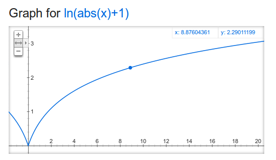
You can see that as the margin of victory gets larger and larger, the multiplier also gets larger and larger, but at a lower rate. I assume they found this equation by guessing what random multipliers worked best for a few sample margin of victories and then graphing a line of best fit.
2) The second problem is autocorrelation Lets say instead of two neutral teams playing each other on a neutral field we have two mismatched teams playing each other. We would have four possible outcomes
1)favorite wins small
2)favorite wins big
3)underdog wins small
4)underdog wins big
>>> rate_1vs1(1550,1450,1,20)
(1560.0, 1440.0)
>>> rate_1vs1(1550,1450,14,20)
(1570.0, 1430.0)
>>> rate_1vs1(1450,1550,1,20)
(1460.0, 1540.0)
>>> rate_1vs1(1450,1550,14,20)
(1470.0, 1530.0)
If these outcomes were all equally likely to occur as they are in the example where its two evenly matched teams playing each other there would be no problem. However, 1550 vs 1450 matchup has a 64% favorite win probability and a 36% underdog win probability. You can use historical averages to see that 64% win % converts to about a 4 point favorite. How often do 4 point favorites lose or win by 7+ points? 4 point favorites win by 7+ points about 40% of the time and lose by 7+ points about 17% of the time. We get the following outcome probabilities
1)favorite wins small 24%
2)favorite wins big 40%
3)underdog wins small 19%
4)underdog wins big 17%
So what is the favorite’s expected ratings after this game is played?
1560 * .24 + 1570 * .40 + 1540 * .19 + 1530 * .17 = 1555.1
But this is wrong. The favorite’s expected rating should actually be 1550, because that is what the team started out rated at. To account for this you need to use a larger k multiplier when the underdog wins big and a smaller k multiplier when the favorite wins big. 538 uses the equation (2.2/((ELOW-ELOL)*.001+2.2)) graphed below as what we’ll call the auto correlation adjustment multiplier or corr_m.
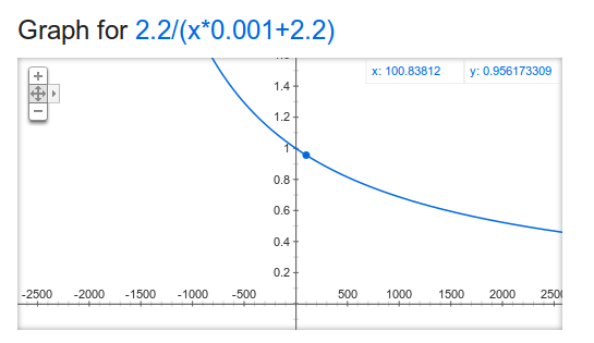
Plugging in our values, when the favorite wins we have 2.2/(100*.001+2.2) = 0.956 and when the underdog wins we have 2.2/(-100*.001+2.2) = 1.048. Our rewritten elo rating function will be
def rate_1vs1(p1, p2, mov=1, k=20, drawn=False):
    k_multiplier = 1.0
    corr_m = 1.0
    if mov >= 7:
        k_multiplier = 2.0
        corr_m = 2.2 / ((p1 - p2)*.001 + 2.2)
    rp1 = 10 ** (p1/400)
    rp2 = 10 ** (p2/400)
    exp_p1 = rp1 / float(rp1 + rp2)
    exp_p2 = rp2 / float(rp1 + rp2)
    if drawn == True:
        s1 = 0.5
        s2 = 0.5
    else:
        s1 = 1
        s2 = 0
    new_p1 = p1 + k_multiplier * corr_m * k * (s1 - exp_p1)
    new_p2 = p2 + k_multiplier * corr_m * k * (s2 - exp_p2)
    return new_p1, new_p2
Our new ratings
>>> rate_1vs1(1550,1450,1,20)
(1560.0, 1440.0)
>>> rate_1vs1(1550,1450,14,20)
(1569.1304347826087, 1430.8695652173913)
>>> rate_1vs1(1450,1550,1,20)
(1460.0, 1540.0)
>>> rate_1vs1(1450,1550,14,20)
(1470.952380952381, 1529.047619047619)
And our new expected rating for p1 is 1560 * .24 + 1569 * .40 + 1540 * .19 + 1529 * .17 = 1554.5
It’s not perfect, but its closer to what it’s true value should be. You could further adjust the corr_m equation or adjust the k_multiplier to optimize your own custom Elo rating system, but this is left as an exercise for the reader.
3) Ratings inflation/deflation.
This is actually not a problem if you’re trying to make predictions in real time. It only matters if you’re a journalist writing an opinion piece on “who’s the greatest of all time?” It is also noteworthy that ratings inflation or deflation will only occur in sports where teams join and leave the league frequently. As long as the # of total points in the league / # of teams in the league ~= 1500 there is no inflation or deflation. In team sports it’s usually not a problem. Expansion teams will come into the league with 1500 points and usually defunct teams are relocated not discontinued so their points can follow them to their new city. For individual sports like boxing or tennis however where new people join the league and old people retire all the time it can be factor to consider when making historical comparisons.
4) Not every win is the same.
This can easily be accounted for with changing k values for games. In chess when established players play each other the match will have a low k value where as when newcomers play they will have a large k value. If you’re using a previous season’s NFL ratings to predict a new season’s games, you should probably have a higher k value for week 1 games than week 14 because its a new season and the ratings should change more quickly based on a single early game rather than a game late in the season where you can be more confident in how good a team really is. For example, if we wanted to use a 50% larger k value for a game, we would just pass in a k value of 30 instead of 20.
>>> rate_1vs1(1500,1500,1,30)
(1515.0, 1485.0)
5) They don’t account for injuries/personnel changes.
This is very similar to the adjustments made in #1. If a team has an injury to QB you should lower their team rating going into a game, where as if their starting QB is coming back from injury you should raise their rating.